
Table of contents
• Preface
• Grouping
Preface
R based open-source collection of scripts called OUKS (Omics Untargeted Key Script) providing comprehensive nine step LC-MS untargeted metabolomic profiling data processing toolbox.
The session info snapshot, information about used packages with comments and scripts are available from https://github.com/plyush1993/OUKS. Each script consists of contents, comments, references and notes in places where functions should be adjusted for experimental parameters (usually “# adjust to your data”). Working directory was set in each script by setwd function, all data tables were loaded into environment in csv format.
Description and instruction for every function can be obtained by the code: ?function. Self-written functions are commented in the script. We utilized a special format for the name of every experimental injection file: “150. qc30 b6 QC30.CDF” for QC sample and “167. s64_2 b7 MS 45.CDF” for study file. Thus, the first value is a run order, then the index of sample with repeat number, batch value and clinical/experimental ID (or QC ID). This form allows to obtaining key information directly from the file name and automatically constructs data frame in the R environment. You can load a similar table to your environment manually if you prefer a different name format.
Raw data (.CDF format) and table with metadata (“metadata.csv”) are the only requirements to reproduce the entire code and are available from Metabolomics Workbench, study ID: ST001682. Other input files (.csv data tables and .R/.RData files) can be generated in the appropriate script or downloaded from the GitHub repository. The entire processing scheme can be easily adapted to the researcher’s needs and their raw data or data tables. The information about used packages and some troubleshooting procedures are described in “installed packages.docx” file. Other useful information, references and significant additions are listed below by each script file name.
To reproduce any script code, download all files to the working directory folder, set the working directory and load (install) the corresponding packages. The R Markdown document and reports files were provided as an example to reproduce the OUKS code script (available in “Report (Rmd)” folder).
The only requirements are to be familiar with the basic syntax of the R language, PC with Internet connection and Windows OS (desirable), RStudio and R (≥ 4.1.2).
OUKS has been published in the Journal of Proteome Research. If you use this software to analyze your own data, please cite it as below, thanks:
New features include:
5 QC-based correction methods (KNN, DT, BT, CTB, XGB) [code]
2 additional QC-based correction methods (GAM) [code] + [script] + [package]
2 biological adjusting methods (GAMM/GAM) [code]
Quick access to datasets:
ds <- as.data.frame(fread("https://raw.githubusercontent.com/plyush1993/OUKS/main/Datasets%20(csv)/8%20peaks.csv"))
meta <- as.data.frame(fread("https://raw.githubusercontent.com/plyush1993/OUKS/main/Datasets%20(csv)/metadata.csv"))
Please send any comment, suggestion or question you may have to the author (Dr. Ivan Plyushchenko), email: plyushchenko.ivan@gmail.com.
Randomization
All samples were analyzed at random order to prevent systematic bias [1,2]. Each analytical batch consisted of ten samples in two technical repeats (repeat samples were acquired after last tenth sample and repeats were analyzed at the same order as first repeat). The QC samples were acquired at the beginning of the batch and after every five injections (overall five QC samples for each batch). The code generates a random sequence of samples in accordance with the user’s conditions: the number of samples, technical and biological repeats and batch size.
Integration
In our case 311 injects in 13 batches were acquired. All raw data were stored in a specific folder. Seven injects were selected for integration and alignment parameters optimization via IPO [3] (1 (batch 1, 1st QC from 5), 75 (3, 5), 101 (5, 1), 163 (7, 3), 219 (9, 4), 257 (11, 2), 311 (13, 3 of 3)) in order to decrease time of computing. QC samples spanning all study were randomly selected (at the beginning, end and middle of batch).
Best parameters were selected for XCMS processing [4] according to IPO optimization. Only bw and minfrac parameters were manually checked according to [5,6]. The “bw” parameter did not introduce any benefits in terms of the number of peaks. The decreasing of “minfrac” parameter sequentially increase the number of peaks and “minfrac” was finally set equal to minimum proportion of the smallest experimental group (0.2 for QC group). Peaks integration, grouping and retention time alignment were performed for all 311 sample injections (without blank injections). The final peak table was described by total number of peaks and fraction of missing values.
Warpgroup algorithm [7] for increasing of precision XCMS results integration was also tested. However, time of computing was approximately 6 days (test was performed via 5 random peak groups). ncGTW algorithm [8] for increasing of precision XCMS alignment results was also implemented. Alternative way is checking different “bw “values. cpc package [9] for filtering low quality peaks was added.
Other approaches for XCMS parameters selection (Autotuner [10] in semi-automatic mode and MetaboAnalystR [11], Paramounter [12] in automatic) were also implemented as alternative options. All .RData files that are needed to implement the Paramounter algorithm can be loaded from the GitHub repository.
Also, old version of XCMS functions (in consistent with xcmsSet objects instead of XCMSnExp objects in recent version) and new capabilities, that are provided by “refineChromPeaks”, “groupFeatures” functions and subset-based alignment, were integrated into the script. Data smoothing and refinement of the centroid’s m/z values (by MSnbase package) were appended.
Target peak integration in EIC chromatograms is also available.
Imputation
Artifacts checking was performed via MetProc [13] which is based on the comparison of missing rates (all peaks were retained). Automatic missingness type determination and imputation were implemented by [14] or by custom function.
Eighteen methods of missing value imputation (MVI) are available for previously obtained peak table, closely to [15]: the half minimum, other univariate MVI methods: converting NA values into the one single number (for example, 0), replacing by mean or median or minimum values, minSample and by random generated numbers, KNN (k-nearest neighbors), PLS (partial least squares), PPCA (probabilistic principal component analysis, or other PCA-based: BPCA, SVD), CART (Classification and Regression Tree), three types of RF (random forest), tWLSA multivariate MVI algorithm [16] and QRILC (quantile regression for the imputation of left-censored missing data) algorithms were implemented for data table without any NA values and with randomly introducing NA values (proportion of introducing was equal to proportion of NA in the original dataset) [17]. The best algorithm was selected by the normalized root-mean-square error (NRMSE, value between 0 and 1) value close to zero (the RF implementation from missForest package). Sum of squared error in Procrustes analysis on principal component scores (minimal value required) and correlation coefficient (maximum value required) were implemented as other quality metrics for MVI. Values for random generation are produced by normal distribution with mean equal to the noise level (which was determined by IPO optimization or set manually) and standard deviation which was calculated from the noise (for example, 0.3*noise).
Correction
34 methods for signal drift correction and batch effects removal were implemented in this work, which include: model-based (WaveICA [18], WaveICA 2.0 [19], EigenMS [20], RUVSeqs family [21,22] (RUVSeqs, RUVSeqg, RUVSeqr), Parametric/Non-Parametric Combat, Ber, Ber-Bagging [23]), internal standards based [24,25] (SIS, NOMIS, CCMN, BMIS), QC metabolites based [25] (ruvrand, ruvrandclust), QC samples based regression algorithms are: cubic smoothing splines [26,27] (in two implementations via pmp and notame packages), local polynomial regression fitting (LOESS) and RF [28] (LOESS and RF in both division and subtraction modes), support vector machine (SVM) [29], least-squares/ robust (LM/RLM) and censored (TOBIT) [30], LOESS or splines with mclust [31], SERRF [32], TIGERr [33], 5 new algorithms each with single, two features and batchwise modes (all also in subtraction/division versions) – KNN (caret package), decision tree (rpart), bagging tree (ipred), XGB (xgboost) and catboost (catboost) gradient boosting, also 2 new QC-GAM (MetCorR) methods and QC-NORM for between batches correction [34]. QC-NORM was implemented in four versions: division-based [34] and subtraction-based [35] and each in a sample-wise or feature-wise manner. Moreover, sequential combinations of methods without consideration of batch number and QC-NORM were also performed. De facto, random forest method is equal to bagging for the regression with only one variable, but due to some differences in trees growing and pruning, modeling results differ.
5 new methods in single division mode were performed according to the equations (1-3):
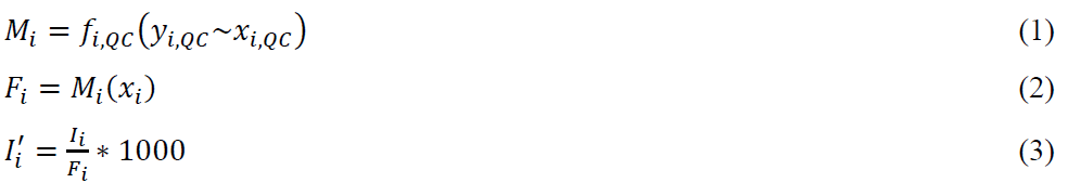 where, i – is the index of metabolite, QC – is the index of QC samples (all samples are denoted without this index), M – is a machine learning model, is fitted by function f, I – is an original intensity vector (dependent variable), x – is a run order vector (independent variable), F – is a vector of predicted values by the model M (correction factor), I’ – is a vector of a corrected intensity values, mean – the function, that generates the mean value from the input vector.
Equations (1-3) are one of the basic algorithms for all QC sample based algorithms for the signal drift correction and are most similar to the statTarget package [28] (changes in multiplying factor). The MetNormalizer package [29] also performs clustering of features via Spearman correlation and the same correction operation (division). Correction algorithm, which is described by the eq. 1-3, was marked as single division mode (“d”).
 where, i – is the index of metabolite, QC – is the index of QC samples (all samples are denoted without this index), I – is an original intensity vector (dependent variable), F – is a vector of predicted values by the model M (correction factor), I’ – is a vector of a corrected intensity values, mean – the function, that generates the mean value from the input vector.
Equation (4) is the modification for equation (3) of previously described algorithm (eq. 1-3), which is called single subtraction mode (eq. 1-2,4; “s”). The same mode was implemented in the BatchCorrMetabolomics [30] and notame [27] packages. Other mode in notame utilizes a correction factor with some changes (including prediction for the 1st QC sample and raw data).
Some QC sample based algorithms consider batch number. Batchwise mode (“bw”) is identical to the two types of single mode (eq. 1-3 division and 1-2,4 subtraction), but each equation was repeated for each batch separately. This implementation is similar to pmp package [26] (the difference with division mode in the correction factor, which includes the median value of the feature) and is closely to batchCorr package [31] (the differences are in the correction factor and clustering features by the mclust algorithm).
Other way is an inclusion batch number into the regression model equation (into eq. 1, as in package BatchCorrMetabolomics [30]). This implementation was called Two Features mode (“tf”) and was implemented both for subtraction and division modes.
Thus, totally 30 algorithms were proposed: each of 5 regression algorithms were implemented in 6 modes (3 (single, “bw”, “tf”) multiplied by 2 (division, subtraction)). In addition, MetCorR is implemented in single subtraction mode and with interaction term with batch. All new correction methods in all modes were written with apply family functions and progress bar.
All .RData files that are needed to implement the SERRF algorithm can be loaded from the GitHub repository.
18 methods for the quality checking and comparison of corrections methods [25, 30, 34-37] are performed, which include: guided principal component analysis (gPCA), principal variance component analysis (PVCA), fraction of features with p-value below the significance level in the ANOVA model, mean Pearson correlation coefficient for QC samples, mean Silhouette score in HCA on PCs scores for QC samples, fraction of features with p-value below the significance level in the One-Sample test (sequential implementation of Shapiro-Wilk normality test and corresponding type of test (t-test or Wilcoxon)) for all QC samples or selected test for each batch separately, fraction of features under the criterion of 30% RSD reproducibility in QC samples, fraction of features under the criterion of 50% D-Ratio between study and QC samples, mean Bhattacharyya distance for QC samples between batches, mean dissimilarity score for QC samples, mean classification accuracy for QC samples after hierarchical clustering on PCs scores, Partial R-square (PC-PR2) method and PCA, hierarchical cluster analysis (HCA), box-plots, relative log abundance (RLA)– plots, correlogram and scatter plot (total intensity versus run order) data projection and visualization. The best correction method should demonstrate the maximum values of the fraction of features under the criterion of 30% RSD reproducibility in QC samples and the mean Pearson correlation coefficient for QC samples. The values of other metrics should be the lowest. PCA, box-plots, scatter plots and HCA dendrogram should show the absence of tendency for the samples to cluster according to batch number or run order, and simultaneously QC samples should be placed almost between study samples.
Annotation
Features in peak table (the output of XCMS processing) were annotated via CAMERA [38], RAMClustR [39], xMSannotator [40] and mWISE [41]. The sr and st parameters in RAMClustR were optimized by functions from [5]. Other settings which include mass detection accuracy in ppm and m/z values and time deviation in seconds were derived from IPO optimized parameters and manual inspection respectively. Annotations should be performed for files in the same folder as for XCMS integration and alignment, xcms objects (“xcms obj … .RData”) should be obtained by user. A search of isotope peaks, adducts, neutral losses and in-source fragments were included in all algorithms. The xMSannotator also considers retention time and database search (HMDB, KEGG, LipidMaps, T3DB, and ChemSpider).
Each algorithm was characterized by a fraction of annotated features. The xMSannotator and mWISE provided the maximum value of annotated ions.
Also, metID [42] can be used for simple databases search from peak table. Databases from (https://github.com/jaspershen/demoData/tree/master/inst/ms2_database) should be copied in “ms2_database” folder in metID library folder.
MetaboAnnotation [43] also can be used for database-based annotation (https://github.com/jorainer/MetaboAnnotationTutorials/releases/tag/2021-11-02).
Filtering
Several most common options are available [1, 27, 35, 44]: RSD based filtering by QC samples, D-Ratio between study and QC samples, annotation based (remove non-annotated features), by descriptive statistics for biological samples (by mean, max, min, median values of the feature or sd), by the fraction of missing values in the feature for biological samples, by the cutoff between median values of feature in QS or biological samples and blanks injections and by the Pearson correlation coefficient for samples (mainly for repeated injections). The mean values for every feature for all repeats are also computed. The mean values for two repeats were obtained in our study.
Normalization
Eight normalization methods are performed [45,46]: mass spectrometry total useful signal (MSTUS), probabilistic quotient normalization (PQN), quantile, median fold change, Adaptive Box-Cox Transformation [47], MAFFIN [48], based on sample-wise descriptive stats and sample-specific factor. Also, several scaling and transformation algorithms are introduced: log transformation, auto- , range- , pareto- , vast- , level- , power-, etc. scaling.
Biological and phenotyping metadata (classification class, age, sex, BMI, etc.) as well as experimental conditions (run order, batch number, etc.) can be adjusted by linear model (LM) [49] or linear mixed effect model (LMM) [50] fitting. Both algorithms were implemented in the study.
The LMM approach fits the model according to a user-defined formula. In this study, model was constructed for each metabolite intensity as an dependent variable; age, class and sex – as fixed effects and batch ID – as a random effect. Then, the original data was employed as input and predicted values from the models were the final output.
 where, i – is the index of metabolite, j – is the index of independent variable j = 1,2, … n (fixed effects), Φ – is a LMM model is fitted by function f, β0 – is the intercept constant, ε – is the random error, β – is the coefficient of the regression model, x – is an independent variable, I – is a dependent variable (a vector of an original intensity values), μ0 – is the random effect, I’ – is a vector of an adjusted intensity values, that was predicted by model Φ.
The LM factorwise approach works in a similar way. At first, linear model was constructed for each metabolite intensity as a dependent variable and other covariates – as independent variables (Age, Sex, Batch, Class, Order in our study). One of the covariates should be noted as a feature of interest (this biological factor was kept, Class in our study). Then, residuals of models were obtained and design matrix was constructed for the feature of interest and constant intercept. For each model, design matrix was multiplied by regression coefficients of intercept and feature of interest and then was summed with residuals. Obtained values were summed with the difference between their mean values and mean values of the original data. The resulted values were the final output.
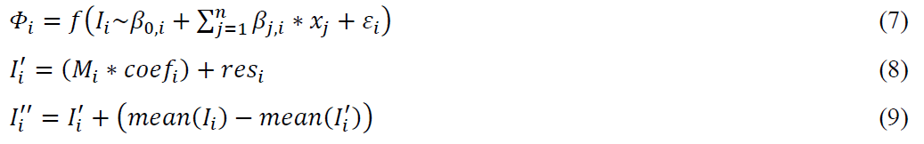 where, i – is the index of metabolite, j – is the index of independent variable j = 1,2, … n (fixed effects), Φ – is a LM model is fitted by function f, β0 – is the intercept constant, ε – is the random error, β – is the coefficient of the regression model, x – is an independent variable, I – is a dependent variable (a vector of an original intensity values), I’ – is a vector of a transformed intensity values, I’’ – is a vector of an adjusted intensity value, M – is a design matrix, that was constructed for the feature of interest and constant intercept, coef – is a vector of regression coefficients of intercept and feature of interest from the model Φ, res – is a vector of the residuals of model Φ, mean – the function, that generates the mean value from the input vector.
Other type of LM adjustment was implemented in similar way to LMM (eq. 5-6 without random effect).
GAM, GAMM [51] adjustment were also realized (as in eq. 5-6).
Five algorithms are utilized for evaluation of normalization methods, including: MA- , Box- , RLA– plots and mean/range of relative abundance between all features [25,52,53]. Biological adjustment methods were tested by classification accuracy via four machine learning (ML) algorithms (RF, linear SVM, nearest shrunken centroids (PAM), PLS), the high value of accuracy indicates successful removing of biological variation. ML parameters are listed in Section 9. PCA modeling was used for visualization of final adjustment/normalization. LM and LMM models were fitted in a similar way as described above (eq. 7,5). The fraction of p-values for the target variable and/or other covariates in the model less than the threshold (0.05) can serve as other character of the adjustment quality (the fraction should be the lowest for covariates and the largest for the target variable).
Grouping
Molecular features from data table after integration and alignment can be clustered (grouped) by different algorithms in order to determine an independent molecular feature and dimensionality reduction. The pmd package [54] performs hierarchical cluster analysis for this purpose (and also provides reactomics). The notame package [27] and CROP algorithm [55] utilize the Pearson correlation coefficient. Final signals represent the largest/mean/median values of features groups.
All .RData files that are needed to implement the CROP algorithm can be loaded from the GitHub repository.
Statistics
Statistical analysis part is divided into several logical blocks. Basic information and principles behind this chapter are available in [56-60]. Calculations are performed with basic functions, if no package is specified.
Outlier detection is performed by calculation of Mahalanobis/Euclidean distance for PCA scores (packages: OutlierDetection, pcaMethods or ClassDiscovery); Hotelling Ellipse with T-squared statistic (HotellingEllipse) and DModX metric (pcaMethods).
Statistical filtration block includes numerous methods for selection of informative variables:
• 1-2). A combination of four ML models with stable feature extraction (SFE) and recursive feature selection (RFS) [61] (packages: caret, tuple). Lists of the top N (50,100, etc) important features from each model were selected according to the model-specific metric in order to perform SFE. The unique variables are subsequently extracted from the set of important features from all models that are matched in at least n times (from 2 to 4 or equal to 50%-100% frequency). RFS with Naïve Bayes (NB) or RF algorithm is applied to subsets of variables after SFE for collection final variable set. The N and n are determined experimentally. Filtration can be performed by SFE only or SFE with RFS. The following parameters were applied when building the models: initial dataset was divided into two subsets by the 10 folds cross-validation with 10 times repeats for internal validation. The hyper-parameters tune length was 10. The four base ML algorithms were implemented: RF, SVM with radial kernel function, PLS and PAM. Only the most important value was tuned in each model (SVM – cost of constraints violation, RF – number of variables at each split, PLS – number of components, PAM – shrinkage threshold). All models were optimized by maximum mean accuracy metric across all cross-validation resampling. RFS was performed by backwards selection between all variables in subset. ML parameters in RFS were equal to those described above.
• 3-4). Consensus/Nested feature selection with multiple filtration criteria [62].
• 5). Filtration by VIP value from PLS (Orthogonal-PLS) model (package: ropls). The filtration threshold is determined experimentally.
• 6). Filtration by permutation importance from RF model (packages: permimp, party). The filtration threshold is determined experimentally.
• 7-8). Filtration by penalized or stepwise logistic regression models (packages: glmnet, MASS). The filtration threshold is determined experimentally.
• 9). Area Under Receiver Operating Characteristic (AUROC) calculations are computed in caret package. The trapezoidal rule is used to compute the area under the ROC curve for each predictor in binary classification. This area is used as the measure of variable importance and for filtration. The problem is decomposed into all pairwise tasks for multiclass outcomes and the area under the curve is calculated for each class pair. The mean value of AUROC across all predictors is directly calculated for binary classification task, for multiclass – at first, sum of AUROC for all groups pairs is determined and is divided by number of class labels and then mean value of AUROC across all predictors is measured. The filtration threshold is determined experimentally.
• 10). Univariate filtering (UVF) is a subsequent implementation of Shapiro-Wilk normality test, Bartlett test of homoscedasticity and Wilcox, Welch, Student tests with Benjamini-Hochberg method for multiple comparison (significance level was set 5% by default). The feature is filtered if significant level is reached between two groups in binary classification and at least any two groups – in multilabel task.
• 11-12). Kruskal-Wallis and t-test can be performed separately. The feature is filtered if significant level is reached.
• 13). Filtration by fold change value. The value is set manually. Fold change calculation for multiclass dataset can be also performed.
• 14). Filtration by moderated t-test [63] (limma package). The significant level is set manually.
• 15-16). Filtration by LM and LMM models (eq. 7,5; packages: MetabolomicsBasics, lme4, lmerTest). The features are filtered by p-value (set manually) for the target variable.
• 17). Filtration by RUV2 algorithm ([64], package NormalizeMets). The p-value cutoff for the target variable is set manually.
• 18). Filtration by Boruta algorithm ([64], package Boruta).
• 19). Filtration by two-dimensional false discovery rate control [66].
• 20). Filtration by removing highly correlated features (package caret). The absolute values of pair-wise correlations are considered. If two variables have a high correlation, the function looks at the mean absolute correlation of each variable and removes the variable with the largest mean absolute correlation. The cutoff for pairwise absolute correlation is set manually.
• 21). Filtration by correlation coefficient. Each variable is compared with vector of target numeric variable. Correlation cutoff is set manually.
Statistical filtration output can be adapted for any combination of filtration algorithms by selection of intersected variables or all unique features.
Another part of “Statistics” script is a classification model task. At first, dataset is divided into training and validation subsets. Then, resampling procedure is determined (bootstrap or cross-validation) and classification metric (ROC or accuracy) is specified (internal validation). In the next part ML model is fitted to training set via caret wrapper function. Hyperparameter tune length is set to 10 and can be changed. The resulted ML model is used for prediction on validation set (external validation) and resulted model overview with resampling statistics are provided. Also, logistic, penalized and stepwise logistic regression (packages: glmnet, MASS) are constructed in similar way. Performance of the models are tested by construction of confusion matrix on training and predicted class labels and ROC analysis. Nested cross-validation [67] is also implemented. Generalized Weighted Quantile Sum (gWQS) Regression [68] is also available as option for classification task. Features can be visualized via box-plot or scatter-plot by groups.
Regression model task is constructed in the same manner as classification task. The differences are as follows: metric is RMSE, MAE or R2; performance is tested by MAE, RMSE, R2 values; optimal subset of variables selection, penalized regression and stepwise regression are performed via leaps, glmnet and MASS packages; visualization is conducted by scatter plot of predicted and training data points. Nested cross-validation is also implemented. gWQS is also available for regression task.
Next block is testing of biomarker set. Features can be visualized via scatter plot by data points and box or violin plots by one or two groups. MANOVA and PERMANOVA (packages: vegan, pairwiseAdonis) procedures are available. Means comparison can be performed as: fold change calculation, t-/moderated t-/Wilcoxon/ Kruskal-Wallis tests, two-way ANOVA and one-way ANOVA (equal to UVF), and volcano plot. In all cases, p-values are adjusted for multiple comparisons.
Metabolomic-Wide association study (MWAS) and analysis of covariance (ANCOVA) are carried out in the form of LM and LMM modeling (eq. 7,5) or similarly by GAM, GAMM and nonlinear dose-response curves (DRC). Also, LM, LMM, GLM, GLMM and correlation analysis are available (with Class as dependent variable) [69].
Signal modeling can be implemented by LM, LMM, GAM, GAMM and some other nonlinear functions for Dose-Response curve (DRC) analysis.
N-factor analysis is implemented by LM/LMM/GAM/GAMM/DRC modeling equally to MWAS/ANCOVA and Signal modeling case. ANOVA-simultaneous component analysis (ASCA, package MetStaT, [70]) is also accessible as an option for multiway analysis, two-way ANOVA, PLS, sPLS, two-dimensional false discovery rate control, PVCA and PC-PR2.
Analysis of repeated measures is performed by LM/LMM/GAM/GAMM/DRC modeling (eq. 7,5) and multilevel sPLS algorithm (package mixOmics, [71]).
Time series or longitudinal analysis is introduced by LM/LMM/GAM/GAMM/DRC modeling (eq. 7,5), ASCA and multivariate empirical Bayes statistics (package timecourse, [72]). Also, dose-response modeling is available (DRomics [73], TOXcms [74]), profile modeling by LMM Splines (timeOmics [75]), pharmacokinetic analysis (polyPK, [76]) and PVCA, PC-PR2.
Multivariate data visualization and projection is provided by unsupervised data analysis. PCA, HCA, k-means clustering (all in packages: factoextra, FactoMineR, dendextend), HCA on PCA scores, heatmap (package pheatmap), t-distributed stochastic neighbor embedding (packages Rtsne, Rdimtools), other methods (DBSCAN, HDBSCAN, Spectral Clustering, UMAP, MCLUST, MDS, LLE, IsoMap, Laplacian Score, Diffusion Maps, kernel PCA, sparse PCA, ICA, FA, NMF, PAM, CLARA, Fuzzy Clustering by dbscan, umap, NMF, Rdimtools, dimRed packages) and validation with optimization of clustering (Dunn index, silhouette analysis, gap stats, Rand index, p-value for HCA, classification accuracy, etc.; packages: NbClust, clustertend, mclust, clValid, fpc, pvclust) are available as an options for unsupervised data projection.
Correlation analysis is represented by computing correlation matrix and correlograms (packages: Hmisc, corrplot, psych).
Distance analysis part allows to calculate distance matrix for observations or features by distance metrics (Euclidean, maximum, Manhattan, Canberra, binary or Minkowski) or correlation and plot heatmap.
In the next section, effect size (Cohen’s d and Hedges’g) and power analysis with sample size calculation are available (packages: effectsize, pwr).
References
- Pezzatti, Julian, et al. “Implementation of liquid chromatography-high resolution mass spectrometry methods for untargeted metabolomic analyses of biological samples: A tutorial.” Analytica Chimica Acta 1105 (2020): 28-44.
- Dudzik, Danuta, et al. “Quality assurance procedures for mass spectrometry untargeted metabolomics. a review.” Journal of pharmaceutical and biomedical analysis 147 (2018): 149-173.
- Tautenhahn, Ralf, Christoph Boettcher, and Steffen Neumann. “Highly sensitive feature detection for high resolution LC/MS.” BMC bioinformatics 9.1 (2008): 504.
- Libiseller, Gunnar, et al. “IPO: a tool for automated optimization of XCMS parameters.” BMC bioinformatics 16.1 (2015): 118.
- Fernández-Ochoa, Álvaro, et al. “A Case Report of Switching from Specific Vendor-Based to R-Based Pipelines for Untargeted LC-MS Metabolomics.” Metabolites 10.1 (2020): 28.
- Albóniga, Oihane E., et al. “Optimization of XCMS parameters for LC–MS metabolomics: an assessment of automated versus manual tuning and its effect on the final results.” Metabolomics 16.1 (2020): 14.
- Mahieu, Nathaniel G., Jonathan L. Spalding, and Gary J. Patti. “Warpgroup: increased precision of metabolomic data processing by consensus integration bound analysis.” Bioinformatics 32.2 (2016): 268-275.
- Wu, Chiung-Ting, et al. “Targeted realignment of LC-MS profiles by neighbor-wise compound-specific graphical time warping with misalignment detection.” Bioinformatics 36.9 (2020): 2862-2871.
- Pirttilä, Kristian, et al. “Comprehensive Peak Characterization (CPC) in Untargeted LC-MS Analysis.” Metabolites 12.2 (2022): 137.
- McLean, Craig, and Elizabeth B. Kujawinski. “AutoTuner: high fidelity and robust parameter selection for metabolomics data processing.” Analytical chemistry 92.8 (2020): 5724-5732.
- Pang, Zhiqiang, et al. “MetaboAnalystR 3.0: Toward an optimized workflow for global metabolomics.” Metabolites 10.5 (2020): 186.
- Guo, Jian, Sam Shen, and Tao Huan. “Paramounter: Direct Measurement of Universal Parameters To Process Metabolomics Data in a “White Box”.” Analytical Chemistry (2022).
- Chaffin, Mark D., et al. “MetProc: separating measurement artifacts from true metabolites in an untargeted metabolomics experiment.” Journal of proteome research 18.3 (2018): 1446-1450.
- Dekermanjian, Jonathan P., et al. “Mechanism-aware imputation: a two-step approach in handling missing values in metabolomics.” BMC bioinformatics 23.1 (2022): 1-17.
- Wei, Runmin, et al. “Missing value imputation approach for mass spectrometry-based metabolomics data.” Scientific reports 8.1 (2018): 1-10.
- Kumar, Nishith, Md Hoque, and Masahiro Sugimoto. “Kernel weighted least square approach for imputing missing values of metabolomics data.” Scientific reports 11.1 (2021): 1-12.
- Di Guida, Riccardo, et al. “Non-targeted UHPLC-MS metabolomic data processing methods: a comparative investigation of normalisation, missing value imputation, transformation and scaling.” Metabolomics 12.5 (2016): 93.
- Deng, Kui, et al. “WaveICA: A novel algorithm to remove batch effects for large-scale untargeted metabolomics data based on wavelet analysis.” Analytica chimica acta 1061 (2019): 60-69.
- Deng, Kui, et al. “WaveICA 2.0: a novel batch effect removal method for untargeted metabolomics data without using batch information.” Metabolomics 17.10 (2021): 1-8.
- Karpievitch, Yuliya V., et al. “Metabolomics data normalization with EigenMS.” PloS one 9.12 (2014): e116221.
- Risso, Davide, et al. “Normalization of RNA-seq data using factor analysis of control genes or samples.” Nature biotechnology 32.9 (2014): 896-902.
- Marr, Sue, et al. “LC-MS based plant metabolic profiles of thirteen grassland species grown in diverse neighbourhoods.” Scientific data 8.1 (2021): 1-12.
- Bararpour, Nasim, et al. “DBnorm as an R package for the comparison and selection of appropriate statistical methods for batch effect correction in metabolomic studies.” Scientific reports 11.1 (2021): 1-13.
- Drotleff, Bernhard, and Michael Lämmerhofer. “Guidelines for selection of internal standard-based normalization strategies in untargeted lipidomic profiling by LC-HR-MS/MS.” Analytical chemistry 91.15 (2019): 9836-9843.
- Livera, Alysha M. De, et al. “Statistical methods for handling unwanted variation in metabolomics data.” Analytical chemistry 87.7 (2015): 3606-3615.
- Kirwan, J. A., et al. “Characterising and correcting batch variation in an automated direct infusion mass spectrometry (DIMS) metabolomics workflow.” Analytical and bioanalytical chemistry 405.15 (2013): 5147-5157.
- Klåvus, Anton, et al. ““Notame”: Workflow for Non-Targeted LC–MS Metabolic Profiling.” Metabolites 10.4 (2020): 135.
- Luan, Hemi, et al. “statTarget: A streamlined tool for signal drift correction and interpretations of quantitative mass spectrometry-based omics data.” Analytica chimica acta 1036 (2018): 66-72.
- Shen, Xiaotao, et al. “Normalization and integration of large-scale metabolomics data using support vector regression.” Metabolomics 12.5 (2016): 89.
- Wehrens, Ron, et al. “Improved batch correction in untargeted MS-based metabolomics.” Metabolomics 12.5 (2016): 88.
- Brunius, Carl, Lin Shi, and Rikard Landberg. “Large-scale untargeted LC-MS metabolomics data correction using between-batch feature alignment and cluster-based within-batch signal intensity drift correction.” Metabolomics 12.11 (2016): 173.
- Fan, Sili, et al. “Systematic error removal using random forest for normalizing large-scale untargeted lipidomics data.” Analytical chemistry 91.5 (2019): 3590-3596.
- Han, Siyu, et al. “TIGER: technical variation elimination for metabolomics data using ensemble learning architecture.” Briefings in Bioinformatics (2022).
- Sánchez-Illana, Ángel, et al. “Evaluation of batch effect elimination using quality control replicates in LC-MS metabolite profiling.” Analytica chimica acta 1019 (2018): 38-48.
- Broadhurst, David, et al. “Guidelines and considerations for the use of system suitability and quality control samples in mass spectrometry assays applied in untargeted clinical metabolomic studies.” Metabolomics 14.6 (2018): 1-17.
- Caesar, Lindsay K., Olav M. Kvalheim, and Nadja B. Cech. “Hierarchical cluster analysis of technical replicates to identify interferents in untargeted mass spectrometry metabolomics.” Analytica chimica acta 1021 (2018): 69-77.
- Fages, Anne, et al. “Investigating sources of variability in metabolomic data in the EPIC study: the Principal Component Partial R-square (PC-PR2) method.” Metabolomics 10.6 (2014): 1074-1083.
- Kuhl, Carsten, et al. “CAMERA: an integrated strategy for compound spectra extraction and annotation of liquid chromatography/mass spectrometry data sets.” Analytical chemistry 84.1 (2012): 283-289.
- Broeckling, Corey David, et al. “RAMClust: a novel feature clustering method enables spectral-matching-based annotation for metabolomics data.” Analytical chemistry 86.14 (2014): 6812-6817.
- Uppal, Karan, Douglas I. Walker, and Dean P. Jones. “xMSannotator: an R package for network-based annotation of high-resolution metabolomics data.” Analytical chemistry 89.2 (2017): 1063-1067.
- Barranco-Altirriba, Maria, et al. “mWISE: An Algorithm for Context-Based Annotation of Liquid Chromatography–Mass Spectrometry Features through Diffusion in Graphs.” Analytical Chemistry (2021).
- Shen, Xiaotao, et al. “metID: an R package for automatable compound annotation for LC2MS-based data.” Bioinformatics (2021).
- Rainer, Johannes, et al. “A Modular and Expandable Ecosystem for Metabolomics Data Annotation in R.” Metabolites 12.2 (2022): 173.
- Helmus, Rick, et al. “patRoon: open source software platform for environmental mass spectrometry based non-target screening.” Journal of Cheminformatics 13.1 (2021): 1-25.
- Wu, Yiman, and Liang Li. “Sample normalization methods in quantitative metabolomics.” Journal of Chromatography A 1430 (2016): 80-95.
- Li, Bo, et al. “Performance evaluation and online realization of data-driven normalization methods used in LC/MS based untargeted metabolomics analysis.” Scientific reports 6 (2016): 38881.
- Yu, Huaxu, Peijun Sang, and Tao Huan. “Adaptive Box–Cox Transformation: A Highly Flexible Feature-Specific Data Transformation to Improve Metabolomic Data Normality for Better Statistical Analysis.” Analytical Chemistry (2022).
- Yu, Huaxu, and Tao Huan. “MAFFIN: metabolomics sample normalization using maximal density fold change with high-quality metabolic features and corrected signal intensities.” Bioinformatics 38.13 (2022): 3429-3437.
- António, Carla, ed. Plant metabolomics: Methods and protocols. Humana Press, 2018.
- Wanichthanarak, Kwanjeera, et al. “Accounting for biological variation with linear mixed-effects modelling improves the quality of clinical metabolomics data.” Computational and structural biotechnology journal 17 (2019): 611-618.
- Wood, Simon N. Generalized additive models: an introduction with R. CRC press, 2017.
- Gromski, Piotr S., et al. “The influence of scaling metabolomics data on model classification accuracy.” Metabolomics 11.3 (2015): 684-695.
- Cuevas-Delgado, Paula, et al. “Data-dependent normalization strategies for untargeted metabolomics-a case study.” Analytical and Bioanalytical Chemistry (2020): 1-15.
- Yu, Miao, Mariola Olkowicz, and Janusz Pawliszyn. “Structure/reaction directed analysis for LC-MS based untargeted analysis.” Analytica chimica acta 1050 (2019): 16-24.
- Kouril, Stepán, et al. “CROP: Correlation-based reduction of feature multiplicities in untargeted metabolomic data.” Bioinformatics 36.9 (2020): 2941-2942.
- Li, Shuzhao, ed. Computational Methods and Data Analysis for Metabolomics. Humana Press, 2020.
- Kuhn, Max, and Kjell Johnson. Applied predictive modeling. Vol. 26. New York: Springer, 2013.
- James, Gareth, et al. An introduction to statistical learning. Vol. 112. New York: springer, 2013.
- Lewis, Nigel Da Costa. 100 Statistical Tests in R: What to Choose, how to Easily Calculate, with Over 300 Illustrations and Examples. Heather Hills Press, 2013.
- Kabacoff, Robert. R in Action. Shelter Island, NY, USA: Manning publications, 2011.
- Plyushchenko, Ivan, et al. “An approach for feature selection with data modelling in LC-MS metabolomics.” Analytical Methods 12.28 (2020): 3582-3591.
- Parvandeh, Saeid, et al. “Consensus features nested cross-validation.” Bioinformatics 36.10 (2020): 3093-3098.
- Smyth, Gordon K. “Limma: linear models for microarray data.” Bioinformatics and computational biology solutions using R and Bioconductor. Springer, New York, NY, 2005. 397-420.
- De Livera, Alysha M., et al. “Normalizing and integrating metabolomics data.” Analytical chemistry 84.24 (2012): 10768-10776.
- Kursa, Miron B., and Witold R. Rudnicki. “Feature selection with the Boruta package.” Journal of statistical software 36 (2010): 1-13.
- Yi, Sangyoon, et al. “2dFDR: a new approach to confounder adjustment substantially increases detection power in omics association studies.” Genome biology 22.1 (2021): 1-18.
- Vabalas, Andrius, et al. “Machine learning algorithm validation with a limited sample size.” PloS one 14.11 (2019): e0224365.
- Tanner, Eva M., Carl-Gustaf Bornehag, and Chris Gennings. “Repeated holdout validation for weighted quantile sum regression.” MethodsX 6 (2019): 2855-2860.
- Rodriguez-Martinez, Andrea, et al. “MWASTools: an R/bioconductor package for metabolome-wide association studies.” Bioinformatics 34.5 (2018): 890-892.
- Smilde, Age K., et al. “ANOVA-simultaneous component analysis (ASCA): a new tool for analyzing designed metabolomics data.” Bioinformatics 21.13 (2005): 3043-3048.
- Liquet, Benoit, et al. “A novel approach for biomarker selection and the integration of repeated measures experiments from two assays.” BMC bioinformatics 13.1 (2012): 1-14.
- Tai, Yu Chuan, and Terence P. Speed. “A multivariate empirical Bayes statistic for replicated microarray time course data.” The Annals of Statistics (2006): 2387-2412.
- Larras, Floriane, et al. “DRomics: a Turnkey Tool to support the use of the dose–response framework for omics data in ecological risk assessment.” Environmental science & technology 52.24 (2018): 14461-14468.
- Yao, Cong-Hui, et al. “Dose-response metabolomics to understand biochemical mechanisms and off-target drug effects with the TOXcms software.” Analytical chemistry 92.2 (2019): 1856-1864.
- Bodein, Antoine, et al. “timeOmics: an R package for longitudinal multi-omics data integration.” Bioinformatics (2021).
- Li, Mengci, et al. “polyPK: an R package for pharmacokinetic analysis of multi-component drugs using a metabolomics approach.” Bioinformatics 34.10 (2018): 1792-1